Chapter 3
Helmholtz Equation through BIE
The Helmholtz equation is what the Laplace equation becomes once we let things vibrate. It is the time-harmonic reduction of the wave equation, and it governs acoustic scattering, which is our real target. Much of the machinery carries over unchanged: the fundamental solution is singular in exactly the same way, so the layer potentials and their jump conditions are the ones we already know. What is new is how the problem lives on an unbounded exterior domain. We need the Sommerfeld radiation condition to pin down which solution we mean, and the wave number \(k\) now sits inside the operators we are trying to invert. We first state the sound-soft and sound-hard scattering problems and prove uniqueness of their solutions. We then reformulate them as boundary integral equations and apply the Fredholm alternative, which gives existence, but only for wave numbers that are not eigenvalues of an interior problem. This is a genuine failure and not an artifact of the analysis being loose: at those wave numbers the boundary integral operator really is singular, even though the scattering problem itself is perfectly well-posed. Since we cannot know where these eigenvalues sit for a general scatterer, and numerically we must avoid a whole neighborhood of each, this makes the formulation unpredictable in practice. The remedy is to combine the single- and double-layer potentials into one equation, the combined field integral equation, whose failure modes are governed by the impedance eigenvalue problem from the previous chapter and therefore sit off the real line entirely. We close by choosing the coupling parameter to push those spurious modes as far from the real axis as conditioning allows, and by assembling the resulting solution operators into the Dirichlet-to-Neumann map.
3.1 Acoustic Scattering
Now we turn to looking at the exterior Helmholtz problem or the scattering problem. Say we send a sound (or electromagnetic) wave at an object and we want to see how it interacts with the object. This is the scattering problem. Appropriately, we call the object we probe with the wave a scatterer.
3.1.1 Problem Statement
We will limit ourselves to scatterers and waves in \(\R^2\), but the idea generalizes to higher dimensions and we include a note on how this is carried out.
If we assume the wave speed \(c\) in the medium is constant, then the wave is described by a velocity potential \(U(x,t)\) which satisfies the wave equation
We make the additional assumption standard in classical scattering theory that the acoustic wave is a plane wave and harmonic in time
with \(\omega > 0\). Then the space dependent component, or amplitude, \(u(x)\) satisfies the Helmholtz equation (sometimes called the reduced wave equation)
in the exterior of the curve defining the boundary of the scatterer.
In the scattering problem we denote the Dirichlet and Neumann boundary conditions by the following:
Definition 3.1.1 (Sound Soft Boundary).
Definition 3.1.2 (Sound Hard Boundary).
We call the acoustic wave before it interacts with the scatterer the incidence (or incident) field \(u^{inc}\), and the wave that exists as a result of interacting with \(\partial D\) the scattered field \(u^{scat}\). The total field \(u\) then satisfies
This can be equivalently expressed in polar coordinates
In order to make the solution to the Helmholtz problem unique, we require that the scattered field satisfy the Sommerfeld radiation condition
Definition 3.1.3 (Sommerfeld Radiation Condition).
Essentially, what this says is that the wave can only be a wave going out to infinity. It cannot be a wave coming from infinity. It ensures that far enough away from \(D\), the time dependent scattered field \(U^{scat}(x,t) = u^{scat}(x)e^{- \omega t }\) is an outgoing cylindrical wave
where \(F(\theta)\) is the fart field pattern. We will not do much with the far field pattern in this introduction but it ensures that as we go away from the scatterer at a fixed angle the amplitude decays. Note that the scattered field is the only part of the wave that must satisfy the Sommerfeld radiation condition. The incident wave need not satisfy it.
To recap, if we want to solve the acoustic scattering problem by a plane, time harmonic wave, then we solve for the scattered field \(u^{scat}\). For convention, make the change \(u(x) = u^{scat}(x)\) (then \(u^{tot} = u^{inc} + u\)). Then \(u\) solves
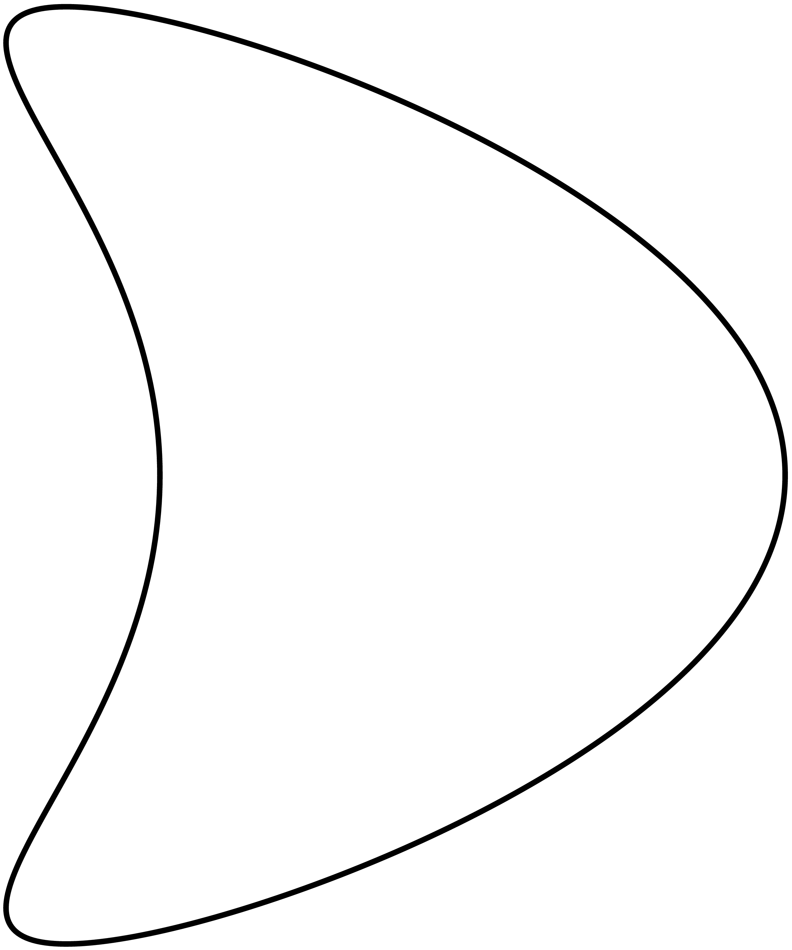
Like many problems in PDEs, if we try to solve the acoustic scattering problem on a circle or sphere, we can use separation of variables to arrive at a closed form solution. We omit the details involving Bessel functions and spherical harmonics. If the reader wishes to indulge oneself, see [2]. An example of the total wavefield when a plane wave incident wavefield interacts with the C-curve, with both sound-soft and sound-hard boundary conditions, is shown in Figure 3.1 and Figure 3.2
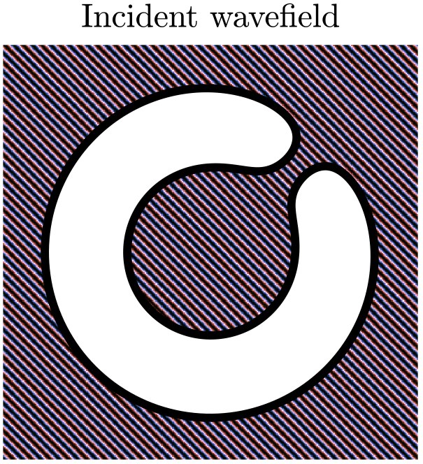
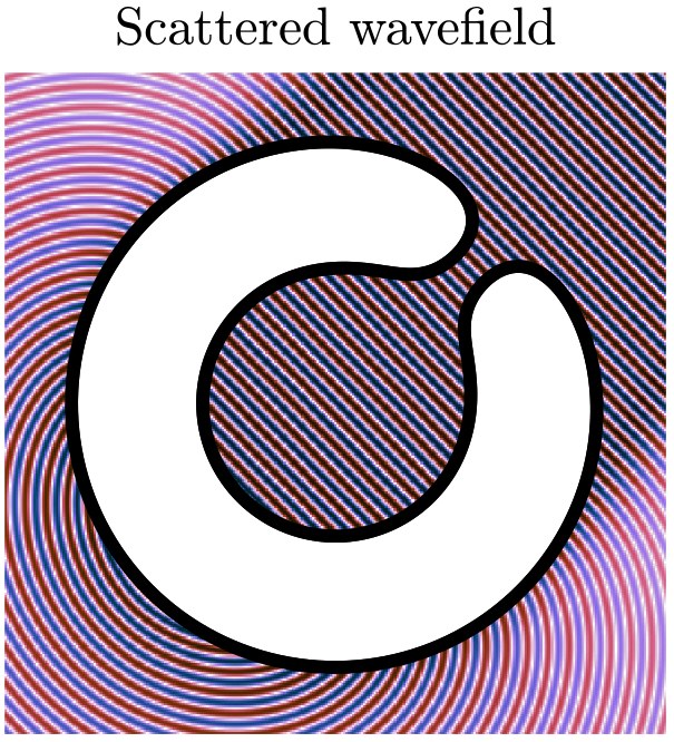
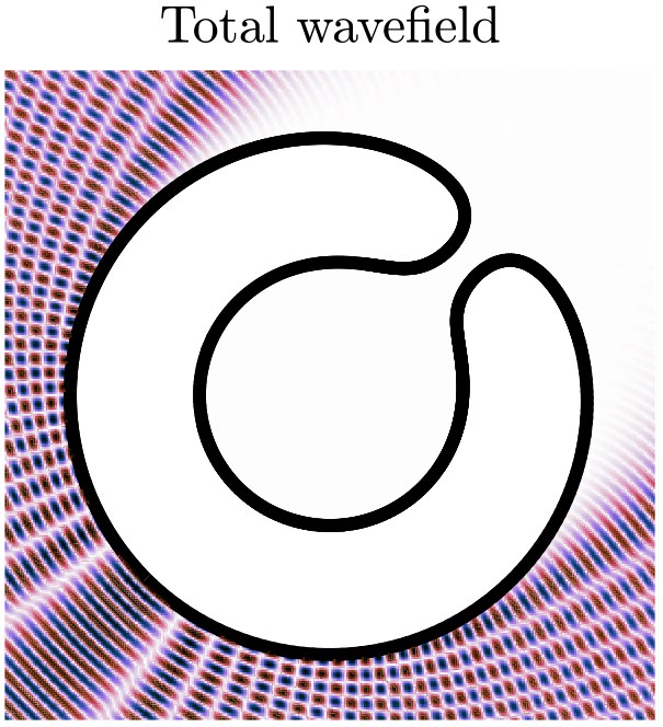
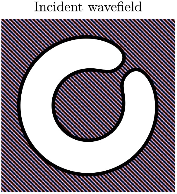
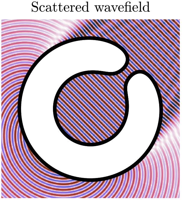
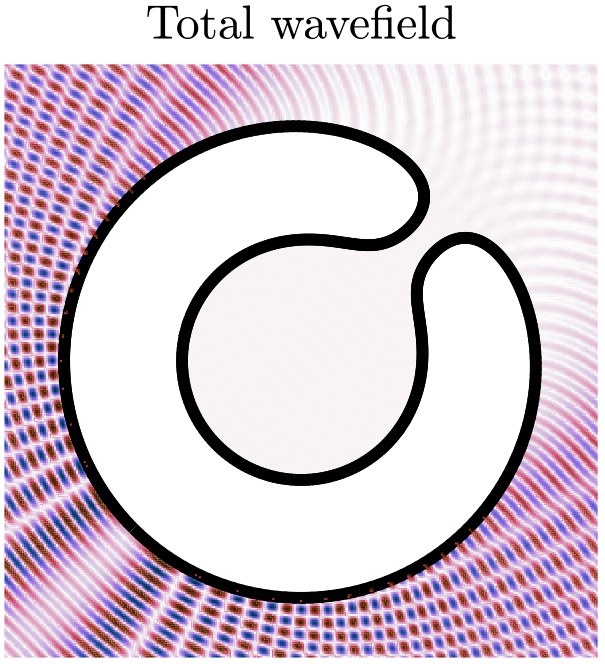
We are interested in the more general case that a scatterer is some curve in \(\R^2\). How do we solve the problem here? Can it be solved at all? If so is the solution unique? The answer to the last two questions is the affirmative, though with more machinery than separation of variables.
Without loss of generality, assume our domain \(D\) contains the origin.
Remark 3.1.4.
For any solution of the Helmholtz equation with Dirichlet boundary data, we would need
and for Neumann boundary data we need
Colton and Kress have shown that (3.3) implies (3.4). Thus we can assume any solution to the Helmholtz equation, and thus the scattering problem, satisfies (3.4).
3.1.2 Solutions on the circle and in the far-field
🚧 Still to be written
This part — a particular solution form for the exterior Helmholtz problem on the circle and in the far-field, presented by Levent Batakci — has not been typed up yet. Check back later!
3.1.3 The Fundamental Solution
Now, like with the Laplace equation, we have a fundamental solution of the Helmholtz equation.
Theorem 3.1.5.
The (radiating) fundamental solution of the Helmholtz equation (3.2) is
where \(H_0^{(1)}\) is the zeroth order Hankel function of the first kind.
Proof.
This follows a similar approach as the fundamental solution to the Laplace equation. Using radial symmetry and using polar coordinates, we obtain the Hankel ODE, due to the Sommerfeld radiation condition we choose the outgoing Hankel functions. The gory details are left to the reader.
In the interest of the double-layer potential, we note that the normal derivative of the fundamental solution is given by
with \(H_1^{(1)}\) the first order Hankel function of the first kind. We now state some facts about the fundamental solution and its normal derivatives that follow from properties of Bessel and Hankel functions.
Observation 3.1.6.
The fundamental solution to the Helmholtz equation (3.5) and its normal derivative (3.6) satisfy the Sommerfeld radiation condition with respect to \(x\) and \(y\).
Observation 3.1.7.
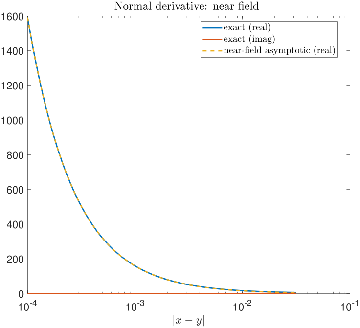
As \(|x-y| \to 0\)
and
Observation 3.1.8.
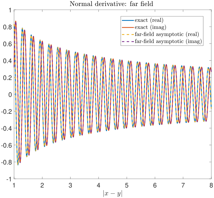
As \(|x-y| \to \infty\) and \(k>0\) real,
and
The fundamental solution and its normal derivative are plotted relative to their asymptotic behavior in Figure 3.3.
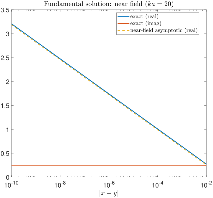
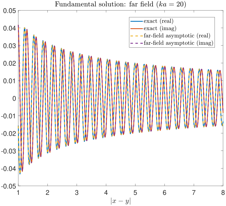
Now we are ready to present a boundary integral formulation of the solution to the Helmholtz equation
Theorem 3.1.9.
Let \(u(x)\) be a solution of the Helmholtz equation in the exterior of \(D\) that satisfies the Sommerfeld radiation condition. Then for \(x \in \R^2 \setminus \overline{D}\)
Proof.
Let \(x \in \R^2 \setminus \overline{D}\) and draw a disk of radius \(\epsilon\) about \(x\) such that the ball is entirely in the exterior of \(D\). That is \(\Omega_{x,\epsilon} = \{ y : |x-y| < \epsilon \}\) and \(\Omega_{x, \epsilon} \cap \overline{D} = \emptyset\).
Draw a second disk \(\Omega\) with radius \(R\) about the origin that encloses both \(D\) and \(\Omega_{x, \epsilon}\).
By Green's second identity, the integral over all the boundaries of \(\partial D, \partial \Omega, \partial \Omega_{x, \epsilon}\) is zero
After the appropriate sign changes to ensure the normal derivative is always pointing outwards of the domain we enclose with the three curves we have explicitly
In the proof, we want to show that the contribution from the integrals over the boundaries of \(\partial \Omega\) and \(\partial \Omega_{x,\epsilon}\) amount to \(0\) and \(-u(x)\), respectively.
On \(\partial \Omega_{x, \epsilon}\) the normal derivative of (3.1.5) is
Taking \(\epsilon \to 0\) in \(\Omega_{x, \epsilon}\) means that on \(\partial \Omega_{x, \epsilon}\), \(|x-y| \to 0\). Further, we can express the coordinate on the boundary with \( y = x + \epsilon \vec{n}\). This change of variables gives us \(ds(y) = \epsilon\,d\vec{n}\)
So we have shown that the contribution from the small circle is exactly \(u(x)\). Next we use the Sommerfeld radiation condition as \(R\to \infty\) to show that
From these two results we get
which gives us
From this theorem we can also make a statement about the solution to the Helmholtz equation on the interior of a domain.
Corollary 3.1.10.
Let \(D\) be any domain and \(u(x)\) a solution of the Helmholtz equation in \(D\). If \(x \in D\) and \(\Omega = \{ y : |x-y| < \epsilon \} \subseteq D\), then
We also have that the fundamental solution \(\phi(x,y)\) is an analytic function with respect to \(x_1, x_2\) such that \(x = (x_1, x_2)\) and where \(x \neq y\). This gives us the following result on the analyticity of \(u(x)\)
Theorem 3.1.11.
Solutions \(u(x)\), with \(x = (x_1, x_2)\) of the Helmholtz equation are analytic functions with respect to \(x_1\) and \(x_2\).
The idea of the proof is similar to the Laplace case and rests on the analyticity of the fundamental solution away from the boundary of the domain.
3.2 Uniqueness of Solutions
We move onto the important issues of existence and uniqueness of solutions to the Helmholtz equations using the machinery of boundary integral equations.
Uniqueness is tackled first, as we will use it in establishing existence. We stress that uniqueness means a single solution. First, we prove a special case of Holmgrem's Theorem.
Theorem 3.2.1.
Let \(u(x)\) be a solution of the Helmholtz solution in the exterior of a domain \(D\) satisfying the Sommerfeld radiation condition and with zero boundary data. Then \(u(x) \equiv 0\) for \(x \in \R^2 \setminus \overline{D}\)
Proof.
We present an outline of the proof. Let \(\Omega\) be a disk centered at the origin containing \(D\) in its interior. We know that \(u(x)\) is analytic in \(\R^2 \setminus \overline{D}\). Thus in \(\R^2 \setminus \Omega\), \(u\) has a series representation
Using asymptotic properties the Bessel and Hankel functions, we show that
which means each coefficient \(a_n\) is zero. This implies \(u(x) \equiv 0\) on \(\R^2 \setminus \Omega\) which in turn implies \(u(x) \equiv 0\) on \(\R^2 \setminus \overline{D}\) by the analyticity of solutions to the Helmholtz equation.
A uniqueness proof follows immediately.
Theorem 3.2.2.
If a solution to the Helmholtz equation exists, then it is unique.
The proof is a standard uniqueness proof in analysis.
Proof.
Assume \(u_1(x)\) and \(u_2(x)\) are both solutions to the Helmholtz equation given some boundary data. Consider the difference equation \(u(x) = u_1(x) - u_2(x)\).
On \(\partial D\), \(u(x) \equiv 0\). From Theorem 3.2.1 we have \(u(x) \equiv 0\) in \(\R^2 \setminus \overline{D}\). Thus \(u_1 = u_2\) in all of \(\R^2 \setminus \overline{D}\) and we are finished.
3.3 Existence of Solutions
With uniqueness squared away we move towards existence. We do so through boundary integral equations and layer potentials. The reader will notice that the arguments presented are similar in spirit to those for the existence of Laplace's equation. Indeed, much is the same between the treatment of the two equations with boundary integral equations, due to their ellipticity.
3.3.1 Layer Potentials
Recall the fundamental solution to the Helmholtz equation from Def 3.1.5
Like in the case of the Laplace equation, we use the fundamental solution to define the single and double layer operators.
Definition 3.3.1 (Single- and double-layer operators).
Given a continuous density function \(\tau\) defined on the boundary \(\partial D\) of a domain \(D\), the integral operators
and
are called the single-layer operator and double-layer operator, respectively. The single and double layer kernels are defined as the fundamental solution and the normal derivative of the fundamental solution, respectively.
and
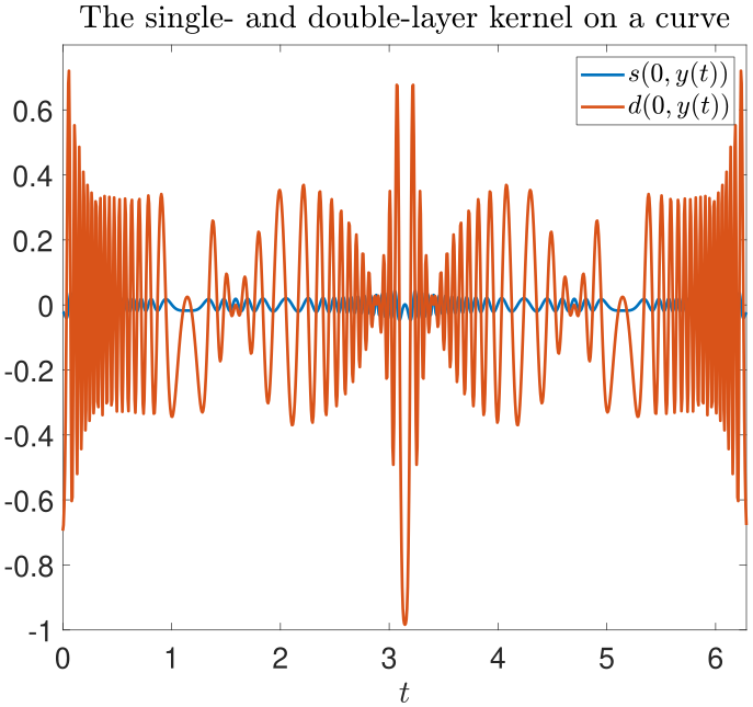
The double- and single-layer kernel for the Helmholtz equation are shown in Figure 3.4 As was the case with the Laplace equation, we can use these operators to define the layer potentials.
Definition 3.3.2 (Single- and double-layer potentials).
Given a continuous density function \(\tau\) defined on the boundary \(\partial D\) of a domain \(D\), we call
the acoustic single-layer potential. Analogously, we call
the acoustic double-layer potential.
Through the single and double-layer potentials, we can express the solution to the Helmholtz equation for interior and exterior problems (i.e. scattering problems) as an integral equation evaluated only on the boundary of the scatterer.
3.3.2 Jump Conditions
In order to define the boundary integral operators and equations we will solve to find solutions to the Helmholtz equation we need to understand how the layer potentials behave as we approach \(\partial D\) from the interior and exterior of the domain. As was the case in Section 2.4.2, the single and double layer kernels for the Helmholtz equation are weakly singular. Thus, the operators \(\mathcal{S}\) and \(\mathcal{D}\) are compact operators! Further, the jump conditions are the same as the Laplace case.
Explicitly, we can extend the double-layer potential from \(\R^2 \setminus \overline{D}\) to \(\partial D\).
Theorem 3.3.3 (Double-layer potential jump condition).
Let \(u(x)\) be the double-layer potential with continuous density \(\tau\) on a domain \(D\) of class \(C^2\). The potential can be extended to \(\partial D\) such that
where the sign \(+\) corresponds to approaching the boundary from the exterior of \(D\) and \(-\) corresponds to approaching the boundary from the interior.
Proof.
The proof follows the same splitting strategy as the proof of the double-layer potential jump condition for the Laplace equation in Theorem Theorem 2.4.4. Indeed we can see that the singularities and their asymptotic behaviors (3.7) and (3.8) are the same as in the double-layer potential of the Laplace equation. The rest of the proof is filled in much the same as in Theorem 2.4.4.
The single-layer potential does not emit a jump condition. It extends unaltered from \(\R^2 \setminus \overline{D}\) to \(\partial D\).
Theorem 3.3.4.
Let \(u(x)\) denote the single-layer potential defined on \(\R^2 \setminus \overline{D}\). The potential can be continuously extended to \(\partial D\) such that
where the integral exists in the improper sense.
3.3.3 Solution Representations
Using the single and double-layer potentials defined on \(\partial D\), we can express solutions to the exterior Dirichlet and Neumann Helmholtz problems. With a focus on the scattering problem, we use the incident field data for the boundary data and require that the solutions satisfy the Sommerfeld radiation condition (3.1.3).
We state these solution representations in the following two theorems.
Theorem 3.3.5.
The acoustic double-layer potential solves the exterior Dirichlet problem
if the density layer \(\tau\) is a solution of the integral equation
In operator notation, this integral equation is given by \((\frac{1}{2}I + \mathcal{D})\tau = -u^{inc}\). The operator \(\frac{1}{2}I + \mathcal{D}\) is a boundary integral operator.
Theorem 3.3.6.
The acoustic single-layer potential solves the exterior Neumann problem
if the density layer \(\tau\) is a solution of the integral equation
In operator notation, this integral equation is given by \((-\frac{1}{2}I + \mathcal{D'})\tau = -\frac{\partial u^{inc}}{\partial \vec n()}\). The operator \(-\frac{1}{2}I + \mathcal{D'}\) is a boundary integral operator.
3.3.4 Fredholm Alternative
These boundary integral operators are of the kind with which we can apply the Fredholm Alternative. In order to do so, we need to understand the nullspaces of the aforementioned boundary integral operators. We will see that these operators have nullspaces which depend on the parameter \(k\), and indeed they emit problematic nullspaces at certain values of \(k\).
Before making a statement on the nullspaces of the boundary integral operators, we will suggestively define
where \(u,v \in C^1(\overline{D})\).
Recall that the nullspace of \(\frac{1}{2}I + \mathcal{D}\) corresponds to the eigenspace of \(\mathcal{D}\) since
which means exactly that \(\tau\) is an eigenfunction of the operator \(\mathcal{D}\). An analogous statement can be made for \(\frac{1}{2}I - \mathcal{D}'\)
This eigenspace-nullspace connection can also be seen in the definitions of (3.17) and (3.18). Consider (3.17). If \(u \in U\), then \(\Delta u = -k^2 u\) in \(D\) subject to the Neumann boundary conditions. Then if \(k^2\) is not an eigenvalue of the interior Neumann problem, the only \(u\) which can satisfy the requirements is \(u \equiv 0\), i.e. \(U = \{ 0 \}\). Alternatively, this means \(k^2\) is an eigenvalue of the negative Laplace operator defined on the interior of the scatterer. Similarly, if \(k^2\) is not an eigenvalue of the interior Dirichlet problem, then \(V = \{ 0 \}\).
The reader might be able to guess the statement we have been building up to. We make the reveal now.
Theorem 3.3.7.
The nullspace of \(\frac{1}{2}I + \mathcal{D}\), \(\bold{N}(\frac{1}{2}I + \mathcal{D})\) is given by \(U\).
Proof.
Assume \(\tau \in \bold{N}(\frac{1}{2}I + \mathcal{D})\). Take \(u(x)\) to be the double-layer potential in \(\R^2 \setminus \partial D\). Define \(u_{+}(x) \) as the limit of \(u(x)\) to \(\partial D\) from the exterior of \(D\).
Then \(u_{+}(x) = 0\). From Theorem 3.2.1 we have that \(u(x) \equiv 0\) for \(x \in \R^2 \setminus D\). Since we have \(u(x) \equiv 0\) outside the scatterer, the normal derivative is zero as we limit to the boundary from the exterior. That is
The normal derivative of the double layer potential is continuous across the boundary \(\partial D\) which gives us
Since we have zero valued Neumann boundary data from the interior of the scatterer, and the double-layer potential is valid for all \(x \in D\), we have that \(u(x)\) solves the interior Neumann problem. The difference of the double-layer potential across \(\partial D\) is exactly the density layer. Combining this with the zero value data in the exterior of \(D\), we have
Writing out the chain explicitly and using that \(u_{-}\) is the double layer potential, we have
which means \(\tau \in U\).
Now to show that \(\tau\in U \implies \tau \in \bold{N}(I + \mathcal{D})\). Assume \(\tau \in U\). Green's second identity gives us
Taking \(x \to \partial D\) we get the boundary integral
which means \(\tau \in \bold{N}(I + \mathcal{D})\)
We present the following result on the nullspace of the operator \(-\frac{1}{2}I + \mathcal{D}'\).
Theorem 3.3.8.
The nullspace of \(-\frac{1}{2}I + \mathcal{D}'\), \(\bold{N}(-\frac{1}{2}I + \mathcal{D}')\) is given by \(V\).
Proof.
Assume \(\tau \in \bold{N}(-\frac{1}{2}I + \mathcal{D}')\). Let \(u(x)\) be the single-layer potential in \(\R^2 \ \partial D\). Define
From the assumption we have \(\frac{\partial u_{+}(x)}{\partial \vec n(x)} = 0\). The uniqueness of the exterior Neumann problem gives us \(u \equiv 0\) for \(x \in \R^2 \setminus \overline{D}\). This implies \(\frac{\partial u_{+}(x)}{\partial \vec n(x)} = 0\). The normal derivative of the single-layer potential is continuous across the boundary \(\partial D\), thus \(\frac{\partial u_{+}(x)}{\partial \vec n(x)} = 0 = \frac{\partial u_{-}(x)}{\partial \vec n(x)}\). From here we see that \(u\) solves the interior Dirichlet problem, thus \(\tau \in V\).
For the reverse, assume \(\tau \in V\). Green's first theorem gives us
So \(v(x)\) is the single-layer potential on the boundary. Then \(v(x) = u_{-}(x)\) Limiting to the boundary, we have
With some algebra we see
Thus \(\tau \in \bold{N}(-\frac{1}{2}I + \mathcal{D}')\).
Finally, with the nullspaces defined for the boundary integral operators which the density layers must satisfy to solve an exterior problem, we can use the Fredholm alternative to state the unique existence of solutions.
Theorem 3.3.9 (Unique Existence of Solutions to Exterior Dirichlet Problem).
The exterior Dirichlet problem as stated in Theorem 3.3.5 is uniquely solvable when \(k\) is not an eigenvalue of the interior Neumann problem.
Proof.
Follows immediately from the Fredholm alternative and Theorem 3.3.7.
Theorem 3.3.10 (Unique Existence of Solutions to Exterior Neumann Problem).
The exterior Neumann problem as stated in Theorem 3.3.5 is uniquely solvable when \(k\) is not an eigenvalue of the interior Dirichlet problem.
Proof.
Follows immediately from the Fredholm alternative and Theorem 3.3.8.
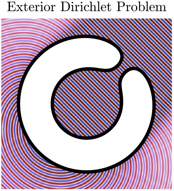
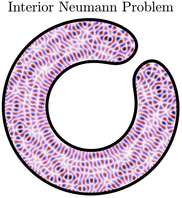
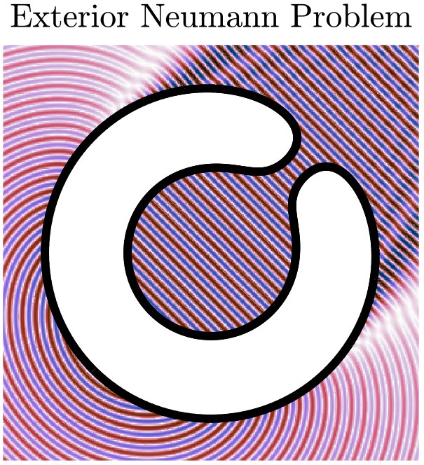
Normally, proving unique existence should leave us satisfied, but these come with a caveat. If we happen to try to solve the exterior problem at an eigenvalue of an interior problem, our boundary integral machinery breaks down, and we are left stranded. Indeed, for a general scatterer we will not know where these interior eigenvalues are, and so solving the exterior problem comes down to a matter of luck. Numerically, the situation is even worse. Instead of only avoiding a problematic wave number, we have to avoid a neighborhood of it. But not all hope is lost! We will see in a subsequent section how to remedy this issue and arrive at a boundary integral formulation that is valid for a much more inclusive set of wave numbers.
3.4 The Combined Field Integral Equations
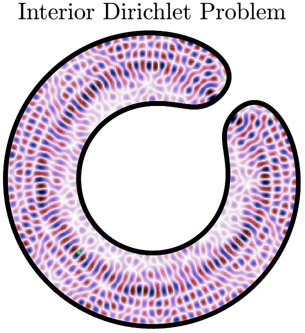
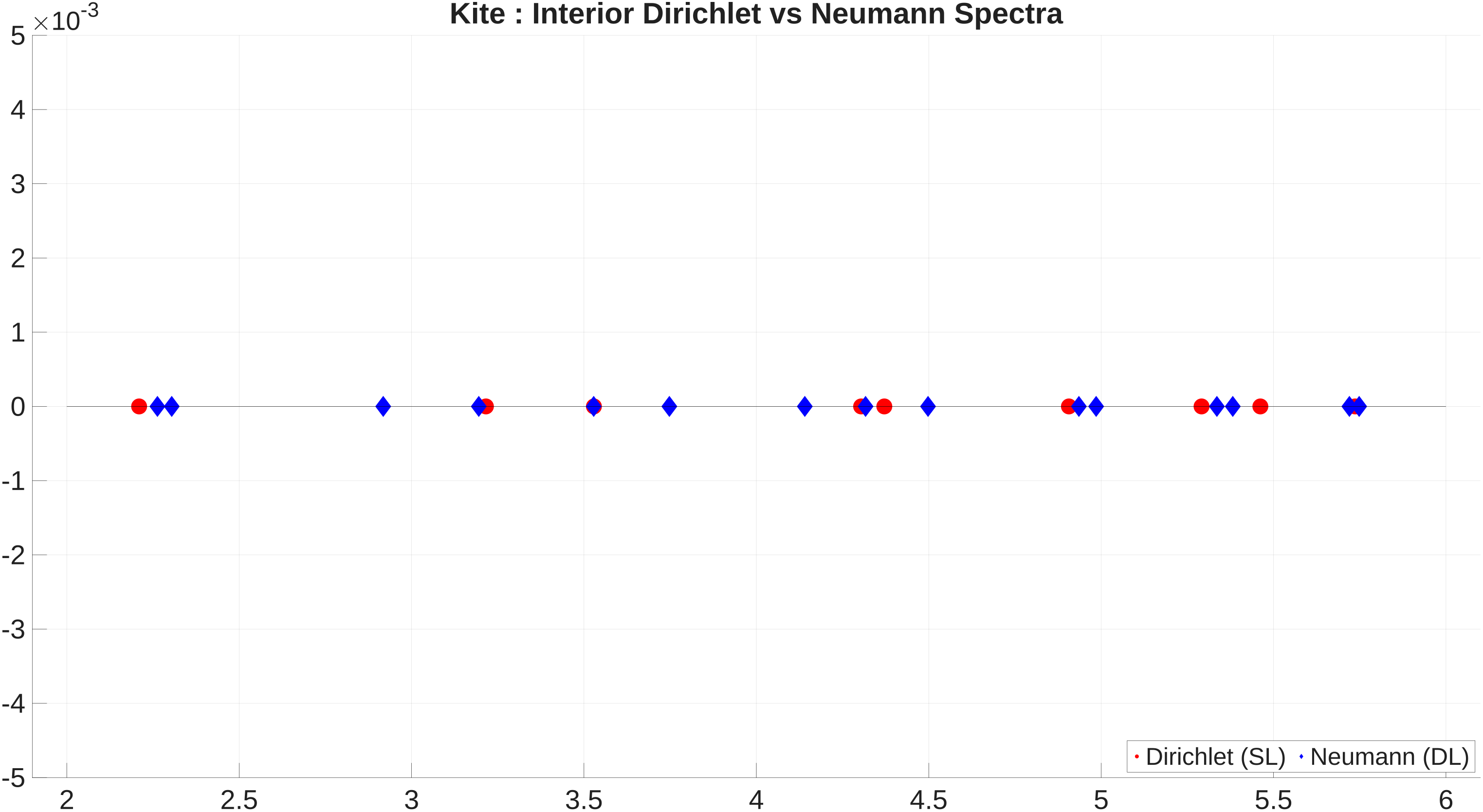
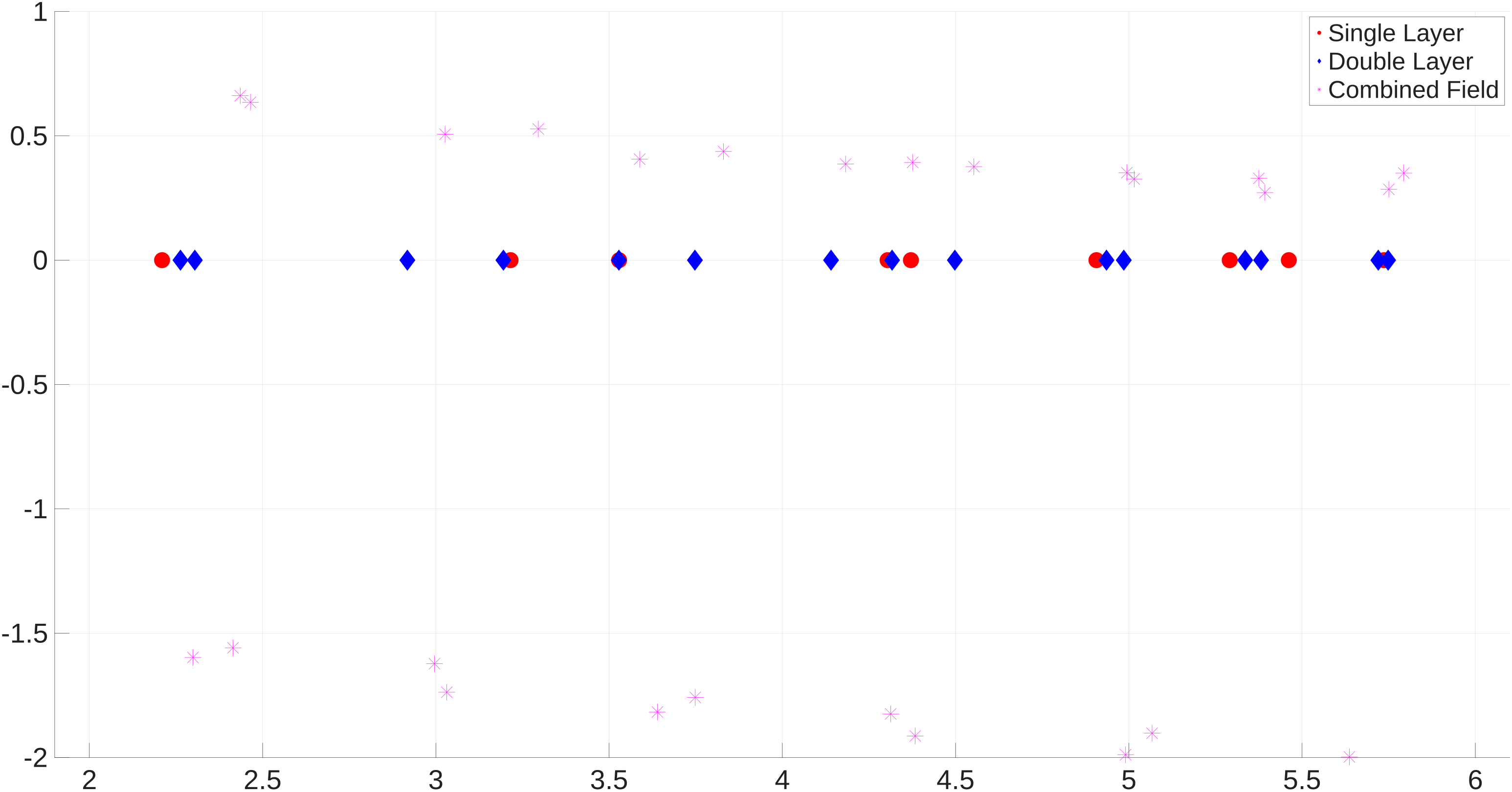
Boundary integral equations for the exterior problems using double- and single-layer operators separately have now been shown to be ill-posed problems when the wave number is an eigenvalue of an interior problem. However, the spectra of the two interior problems seem to be disjoint. While the solution to the Helmholtz equation might not be well-posed through the single-layer potential approach at a certain wave number, the double-layer potential approach will yield a solution. Finding one BIE equation that is well-posed for all real wave numbers rigorously proves the existence of the solution. In a similar vain to Theorem 2.4.6, the Brakhage-Werner Leis, Panich's approach is to use a linear combination of the double- and single-layer potential gives a solution approach to the Helmholtz equation that is well-posed for all real wave numbers [3]. This combination is called the combined field integral formulation. The resulting combined field integral equation (CFIE) is used for exterior problems since we know that the scattering problem observes no resonant modes on the real line, on interior problems, the resonant modes are on the real line and so a BIE where the resonant modes aligns with its ill-posed wave numbers should be chosen. We see this in Figure 3.6.
3.4.1 The sound-soft problem
We state and prove the CFIE for the exterior Dirichlet problem with boundary condition [3, 8].
Theorem 3.4.1.
Let \(D\), be a bounded domain of class \(C^2\) and \(D^C = \R^m\backslash \overline{D}\),
with \(\eta\in\mathbb{R}\) a non-zero coupling parameter and density function \(\tau\in C\) s.t.
is a solution to the exterior Dirichlet problem with boundary condition \(f\).
The proof follows from the jump condition of the double-layer potential. We now show that for any non-zero coupling parameter \(\eta\), the Fredholm integral equation of the second kind (3.20) is injective and through the Fredholm alternative, the inverse exists. While the proof can seem repetitive, it shows where the CFIE fails in the complex plane and indicates a choice of coupling parameter.
Theorem 3.4.2.
Let \(\mathcal{S}\) and \(\mathcal{D}\) be the single- and double-layer operator, then
for any \(\eta \neq 0\) and real wave number \(k\).
Proof.
Let \(\tau\in C\) such that \((\frac{I}{2}+\mathcal{D} - i\eta\mathcal{S})\tau \equiv 0\). That mean that \(u = (\mathcal{D} - i\eta\mathcal{S})\tau\) solve the exterior Helmholtz problem with Dirichlet boundary condition \(u_+\equiv 0\). Due to the uniqueness of the solution, we have that \(u\equiv 0\) in \(D^C\) and therefore \(\frac{\partial u_+}{\partial \vec n}=0\). Now using the jump condition from the double-layer potential (2.6) and normal derivative of the single-layer potential (2.11) (and lack of jumps), we can relate the limiting behavior from the interior \(u_-\) and exterior \(u_+\), of the domain \(D\),
Therefore,
Thus, \(u\) satisfies the Helmholtz equation everywhere but on \(\partial D\) and on the interior of the domain \(D\) has boundary condition \(\frac{\partial u_-}{\partial \vec n} = i\eta u_-\). We have that \(u\) satisfies the Helmholtz BVP with impedance boundary conditions.
This is exactly the eigenvalue problem of the Laplacian with impedance boundary condition seen in Problem 2.5.9, with \(\lambda = k^2\). The eigenvalues depend on the sign of \(\eta\) and no eigenvalues are on the real line! Therefore, when \(k^2\) is not an eigenvalue of the Laplacian with impedance boundary conditions, the solution \(u\) is uniquely \(u\equiv 0\) in \(D\). Since \(k^2\) is real, it cannot be an eigenvalue, hence \(u\equiv 0\), more importantly \(u_-=0\) on \(\partial D\), thus \(\tau = 0\). Therefore
We now know that the CFIE is well-posed for all real wave numbers! However, there are still other wave numbers for which the CFIE is ill-posed while the Helmholtz solution still exists. It is important to know approximately where the wave numbers with ill-posed problems are located [1, 3]. As seen in observation 2.5.10, the sign of the coupling parameter \(\eta\) determines in which half of the complex \(k\)-plane the CFIE is ill-posed. These wave numbers are called spurious modes. They are not wave numbers were the solution to the Helmholtz equation doesn't exists, they are wave numbers where the BIE is ill-posed. Since we know the spurious nodes are only encountered for \(\text{Re}(k)>0\), since \(\text{Im}(k^2)= 2\text{Re}(k)\text{Im}(k)\), we know that when \(\eta\) is chosen to be positive the spurious modes will be in the lower half plane, while when \(\eta\) is negative, the spurious modes will be in the upper half plane. The distance between the spurious nodes and the real line is determined by the value of \(\eta\). Through (2.20) and (2.21), we see that
therefore
For larger \(\eta\), the spurious modes are pushed further into the complex plane. It is seen that \(\eta>1\) is a safe choice, however, we can also take the coupling parameter to be dependent on the wave number for conditioning. Indeed, let \(\eta\) be constant, as the wave number \(k\) grows we see, using Observation 3.1.8,
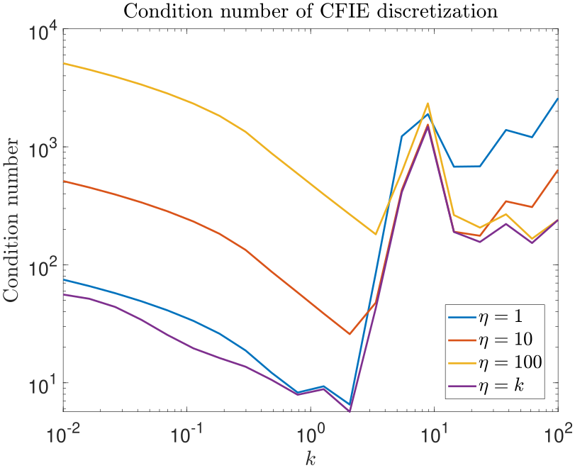
Therefore, if \(\eta\) is constant, as \(k\) grows, we see that we return to the double layer potential which causes the spurious wave number to approach the real line. This leads to a commonly chosen coupling parameter \(\eta = \text{Re}(k)\) [1, 3], we then have that both the single and double layer terms are on the same order of magnitude relative to the wave number. However, as \(k\) grows even further, the CFIE looses the Fredholm integral equation of the second kind's conditioning in numerical approaches. The so-called high-frequency Helmholtz equation comes with many more problems, and is a topic out of the scope of this report [1, 9]. The condition number for various coupling parameters is shown in Figure 3.9.
3.4.2 The sound-hard problem
To solve the sound-hard problem, we define the adjoint to the double layer operator and the hypersingular boundary integral operator, respectively,
and
Let the solution be described as
if the density layer function satisfies
then \(u\) is a solution to the sound-hard scattering problem with boundary condition \(g\). Here the jump condition followed from the normal derivative of the single layer potential and it should be noted that the jump of the double-layer potential does not survive the normal derivative, as discussed in the Laplace chapter. Note that \(\mathcal{T}\) is hypersingular and therefore not compact on \(C(\partial D)\), so Corollary 1.4.18 does not apply directly. Extending the layer operators to \(L^2(\partial D)\) via Theorem 1.4.13 and splitting of the Laplace hypersingular part returns a compact perturbation of an invertible operator. The proof that the integral operator \(\frac{i\eta}{2}I + \mathcal{T} - i\eta \mathcal{D}'\) is invertible is then nearly identical to the proof in Theorem 3.4.2 [3], relying on the uniqueness of the exterior Neumann problem instead of the exterior Dirichlet problem. The BIE is ill-posed at exactly the same spurious modes as the sound-soft problem.
3.4.3 Dirichlet-to-Neumann maps
Being able to solve the sound-soft and sound-hard problem for all real wave numbers \(k\) allows us to describe the behavior at the boundary through a density layer function. This opens up the world of Dirichlet-to-Neumann (DtN) and Neumann-to-Dirichlet (NtD) maps. These maps translates Dirichlet data at the boundary to Neumann data and Neumann data to Dirichlet data, respectively. The DtN map is given by
the NtD map is given by
Note that \(\mathcal{A}_{NtD}= \mathcal{A}_{DtN}^{-1}\), they are not independently-constructed map. The mapping properties stated above are the Hölder ones inherited from the layer operators on \(C(\partial D)\), but the two applications discussed below both treat the DtN map as an operator on energy spaces rather than on Hölder spaces. Both boundary integral operators appearing in \(\mathcal{A}_{DtN}\) have a transposed-kernel partner, obtained by exchanging source and target in the kernel, so Theorem 1.4.13 applies and each is bounded with respect to the \(L^2(\partial D)\) norm. Since \(C(\partial D)\) is dense in \(L^2(\partial D)\), they extend uniquely to bounded operators there, and by Theorem 3.4.2 the extension of \(\frac{I}{2}+\mathcal{D}-i\eta\mathcal{S}\) extends to an injective bounded operator for real \(k\). The DtN map is therefore a bounded operator on \(L^2(\partial D)\), and it is in this setting that the following two interpretations live. Note here that again the choice of \(\eta\) is related to the invertibility of the operators. In the end, the physical DtN and NtD maps are independent of the choice in \(\eta\) on the real line.
Beyond their role in scattering theory, DtN maps are the standard device for turning an unbounded exterior problem into a bounded one. If we want to solve a Helmholtz problem on all of \(\R^m\) numerically, we cannot mesh an infinite domain. Instead we truncate to a bounded region containing all inhomogeneities, and impose \(\mathcal{A}_{DtN}\) as an exact boundary condition on the truncation boundary. This replaces the usual approximate absorbing boundary conditions (Sommerfeld radiation truncated to low order, PML, etc.) with something exact, at the cost of the DtN map itself being nonlocal and expensive to apply [9]. This is the same idea used in non-overlapping domain decomposition methods, where the Schur complement appearing after eliminating interior unknowns on each subdomain is again a DtN map for that subdomain, and iterating between subdomains amounts to iterating on interface data through these maps [9].
Lastly, the DtN map is the central object in a large class of inverse problems. The Calderón problem, the mathematical model behind electrical impedance tomography, asks whether a coefficient (conductivity, or here the wave speed/index of refraction) can be recovered from knowledge of the DtN map alone [3]. Our construction shows that, at least for a fixed known domain \(D\) and real \(k\), this map is well-defined and computable through the CFIE machinery above, which is the starting point for asking such inverse questions numerically.
References
- [1]Alex H. Barnett. MATH 126: Numerical analysis for PDEs and wave scattering. Course notes.
- [2]David Colton. Partial differential equations: an introduction. Courier Corporation, 2004.
- [3]David Colton and Rainer Kress. Inverse Acoustic and Electromagnetic Scattering Theory. Applied Mathematical Sciences, vol. 93, 4th edition, Springer, 2019.
- [8]Rainer Kress, Vladimir Maz'ya, and Vladimir Kozlov. Linear integral equations. Springer, 1989.
- [9]Per-Gunnar Martinsson. Fast direct solvers for elliptic PDEs. SIAM, 2019.