Laplace equation & Layer Potentials

2.1 Harmonic Functions

We say that \(\Delta\) is the Laplacian, and let \(\vec n\) denotes the outward pointing unit normal vector on a curve, we write the normal derivative as \(\frac{\partial u}{\partial \vec n}(x)=\vec n(x)\cdot \nabla u(x)\). Most of the theory of harmonic functions utilize Green's theorems [2, 4]. The first and second Green's theorems are practically a reformulation of Gauss' divergence formula.

The second Green's theorem applied to an harmonic functions (with \(v\equiv 1\)), directly leads us to the corollary that harmonic functions observe net flux zero.

To study harmonic functions we first find the Green's function to the Laplacian, or the fundamental solution to the Laplace equation [4].

As the name suggestions, \(\varphi\) is fundamental to any finding any solution to the Laplace equation in the setting of boundary value problems. The fundamental solution to the Laplace equation also allows us to evaluate a harmonic function through it's behavior at the boundary through Green's formula.

Now to work towards the goals of proving existence and uniqueness of the solution to BVPs with the Laplacian, we note a couple of theorems, the proofs are left to the reader and can be found in [4, 2].

This theorem implicitly states that any harmonic functions is infinitely differentiable at any point \(x\in D\). This allows us to prove the following:

This then lead to the classic Mean Value Theorem [4].

In essence, this theorem state that the function value of a harmonic function \(u\) at \(x\) is equal to the average volume over \(B_r(x)\) and the mean over \(\partial B_r(x)\). This then leads us to the Maximum-Minimum principle [4, 2], which is vital to proving uniqueness of the solution to BVPs with the Laplacian.

Moreover, if \(u\) is harmonic in \(D\) and continuously extends in \(\bar D\), then \(u\) reaches its minimum and maximum on the boundary. The theory of harmonic functions can also be extend to different types unbounded domains. For the purpose of this survey, we are particularly interested in domains \(D^c=\R^m\backslash \bar D\) with \(D\) a bounded domain itself. We refer to \(D\) as the interior domain and \(\R^m\backslash \bar D\) as the exterior domain. The interior and exterior domain are shown in Figure 2.1.

We can extend Green's formula to the unbounded domain by imposing behavior at infinity [3].

2.2 Laplace BVPs

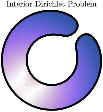
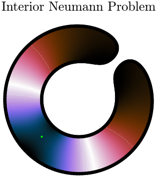
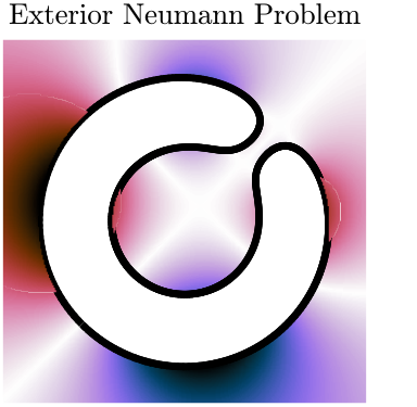
We define four classical Laplace BVPs which are the combinations of interior/exterior with Dirichlet/Neumann boundary conditions [3, 2]. Solutions to these problems are shown in Figure 2.3.

2.3 Solution Uniqueness

We state and loosely prove uniqueness statements of these four problems. It is emphasized that uniqueness of a solution means at most 1 solution exists.

More interesting things happen when the problems do not have a unique solution, but the null-space of the problem is non-trivial, as is the case for the interior Neumann problems. For the purpose of the proof, we define parallel surfaces.

2.4 Solution Existence

The existence proofs are very informative, particularly for numerical methods to solving the Laplace equations through boundary integral equations [3, 9]. For the purpose of existence proofs, we first discuss layer potentials which play a vital role in BIE methods and the rest of this overview. Afterwards, solutions to the Laplace equations are found in terms of these layer potentials by looking at their behavior near the boundary of \(D\) from both sides.

2.4.1 Layer Potentials

We first define two integral operators vital to the rest of this survey [3, 8].

Definition 2.4.1 (Single- and double-layer operators).

Given a density function \(\tau\in C(\partial D)\), the integral operators

\[\mathcal{S}\tau = \int_{\partial D}s(\cdot,y)\tau(y)~\mathrm{d}s(y),\]

and

\[\mathcal{D}\tau = \int_{\partial D}d(\cdot,y)\tau(y)~\mathrm{d}s(y),\]

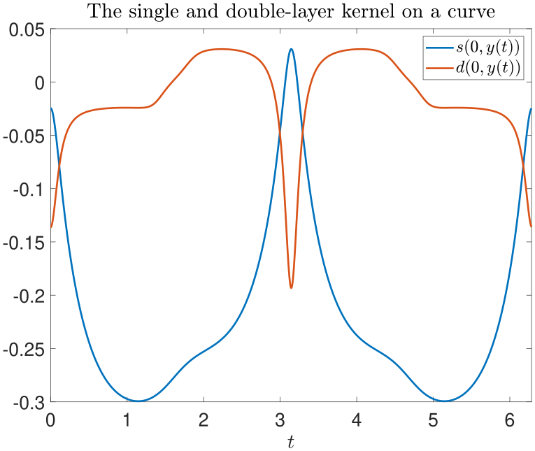
are called, respectively, the single- and double-layer operators. The single- and double-layer kernels are respectively defined as

\[s(x,y) = \varphi(x,y) = \frac{1}{2\pi}\ln\left(\cfrac{1}{|x-y|}\right)\]

and

\[d(x,y) = \frac{\partial \varphi}{\partial \vec n(y)}(x,y) = \frac{1}{2\pi}\frac{\vec{n}(y)\cdot(x-y)}{|x-y|^2},\]

with \(\varphi\) the fundamental solution. The double- and single-layer kernels on the C-curve with target \(x=0\) are shown in Figure 2.2.

We can now define the single- and double layer potentials as

Using the Leibniz Integral Rule, we see that both the single- and double-layer potentials are harmonic functions on domain \(\R^m\backslash \partial D\). Since they are harmonic functions, there might exist specific density function(s) \(\tau\) such that \(u\) and \(v\) satisfy the Laplace BVPs with specific boundary data! Indeed we will prove for a class of boundary data, when a density function can be found, leading to boundary integral equations and the existence of solutions.
Before existence, we touch on how to interpret the single- and double-layer potentials through sources, targets and charges, common terminology in BIEs in scattering theory [9, 1]. The evaluate single-layer potential \(u\) at a target point \(x\), we approximate the single layer integral operator using a quadrature scheme

where \(w(y_j)\) includes quadrature weights and the geometry the boundary \(\partial D\). The value of \(u\) at a target point \(x\) is a sum of various charges coming from source points \(y_j\) with charge \(\varphi(x,y_j)\tau(y_j)w(y_j)\). Since, \(\varphi\) has a singularity when the target and source points are the same, we look at this asif there is a pole, the source points, that eradiates a charge and affects the value of \(u\) at the target point. For this reason, we also call the source point a monopole in this setting. The charge is determined on the distance between \(x\) and \(y_j\) through \(\varphi\) with a boundary \(\partial D\) dependent initial charge from \(w(y_j)\) and \(\tau(y_j)\) describes the charge coming from the value of \(u\) on the boundary itself \(\partial D\). This all combines to one charge coming from one monopole, the full value of \(u\) at the target point is then the sum of all source points with their respective charges. The true single-layer potential then describes the charges coming from an infinite amount of source points.
The double layer potential \(v\) at a target point \(x\) can also be approximated through a quadrature scheme,

To obtain a conceptual grasp, we also approximate the normal derivative through a finite difference formula, for example centered difference,

for \(h\) small. The approximation to the double-layer potential,

can then be interpreted as the affect of two monopoles with charges working in opposite directions and scaled by \(h\), hence \(y_j\) is referred to as a dipole in this setting. The double-layer potential can be seen as vibrations.

2.4.2 Jump conditions

To use the single- and double-layer potentials to solve interior and exterior Laplace problems, a good grasp on the limiting behavior of \(u(x)\) and \(v(x)\) as \(x\) reaches a point on the boundary \(\partial D\). To do so, we first discuss the behavior of the double-layer kernel as \(x\) reaches a point on \(\partial D\) over \(\partial D\). Then we look at the behavior of the single- and double-layer potentials behavior coming from the interior and exterior domain.
Let \(\gamma:[0,L]\to \partial D:t\mapsto \gamma(t)\) be an arclength parametrization of \(\partial D\), \(x(s)=\gamma(s)\), \(y(t)=\gamma(t)\), and \(n(t)\) the outward normal, with Frenet relation \(\gamma''(t)=\kappa(t)\cdot n(t)\), where \(\kappa\) is the curvature of the boundary. We have \(L\) the arc length and \(|\gamma'|\equiv 1\). Taylor expanding the parametrization at \(t\),

Since \(n(t)\cdot\gamma'(t)=0\), by definition, and \(n(t)\cdot\gamma''(t)=\kappa(t)\),

and

Therefore, since \(|\gamma'|\equiv 1\),

Taking \(\epsilon\to 0\),

The kernel has a removable singularity with the limit found. The single-layer kernel has no such limit. This difference leads us to the core engine of boundary integral equations, the jump of the double layer operator from the exterior domain to the interior domain [3]. First we prove Gauss' formula

WE now have all the tools to find the jump of the double layer potential [3, 8].

For the single layer potential, no jump occurs due to the weak singularity. However, it can be used for the interior/exterior Neumann problems. Let \(u(x) = [\mathcal{S}\tau](x) \), we then have that

We define the integral operator to be the adjoint of the double layer potential,

Note that this is an adjoint w.r.t. the bilinear inner product \(\langle\cdot,\cdot\rangle\), and it itself is not a layer potential since it cannot satisfy any Laplace equation. However, similar jump conditions are observed, making them useful for the Neumann problems. Given \(u(x) = [\mathcal{S}\tau](x) \), we can prove

and

This jump is special to the usage of the single layer potential. The jump condition of the double-layer operator does not survive the normal derivative and thus no jump condition is seen for the double-layer potential. In particular,

On the other hand for the single layer potential, since it observes no jump we have that

However, the normal of the single layer potential does observe this jump. Using (2.8) and (2.9), we get

In the interest of future endeavors, we mention two facts on these kernels and future similar kernels [8].
First, we note that if \(\partial D\) is of the class \(C^2\), there exists an constants \(L_1\) and \(L_2\), s.t.,

which is seen through Taylor approximations where \(L_1\) and \(L_2\) are similar to the curvature. This can then be used to see that the double-layer kernel is weakly singular in dimension \(d\geq 2\),

hence \(\mathcal{D}\), and \(\mathcal{D}'\) are compact operators! It is trivial to see that the single layer kernel is also weakly singular and hence \(\mathcal{S}\) is also a compact operator.
Second, with scattering problems in sight, in particular with the Helmholtz equation, we have to note that the fundamental solution to the Helmholtz equation has similar singular behavior at \(|x-y|\to 0\), therefore these jump conditions will translate to the Helmholtz equation with new fundamental solutions.

2.4.3 Solutions through BIEs

The limiting behavior to the boundary now allows to us to reformulate the PDE into a BIE. For the Dirichlet Laplace problems we will be using the jump conditions described in Theorem 2.4.4. For the Interior Dirichlet problems (2.2.1) with boundary condition \(u=f\) on \(\partial D\), we have

For the Exterior Dirichlet problem (2.2.3) with boundary condition \(u=f\) on \(\partial D\), we have

We can also reformulate the Neumann problems to BIEs using the jump conditions (2.9) and (2.8). For the Interior Neumann problem (2.2.2) with boundary condition \(\frac{\partial u}{\partial \vec n}=g\) on \(\partial D\), we have

For the Exterior Neumann problem (2.2.4) with boundary condition \(\Dn u=g\) on \(\partial D\), we have

If we are able to find the density layer function, we are able to find solutions to the Helmholtz equation and thus prove the existence of solutions to the Helmholtz equation. To this end, we have to be able to invert operators like \(\pm\frac{I}{2}+\mathcal{D}\) and \(\pm\frac{I}{2}+\mathcal{D}'\). There are ”direct“ boundary integral formulations that, given Dirichlet boundary data, find Neumann boundary data to then use the Green's formula (2.3). For example, for the Dirichlet problem, we find the Neumann boundary data through

or given Neumann boundary data, we find the Dirichlet boundary data through

While the two do not need to an extra density functions \(\tau\), which comes with it's extra problems, we instead compute the other boundary data. However, an operator is still needs to be inverted and evaluated. In particular, here we must invert a compact operator, or Fredholm integral equation of the first kind \(\mathcal{S}\Dn u\). On the other hand, since \(\mathcal{D}\) and \(\mathcal{D}'\) are compact operators, we have that \(\pm\frac{I}{2}+\mathcal{D}\) and \(\pm\frac{I}{2}+\mathcal{D}'\) Fredholm integral equations of the second kind on which we are able to apply the Fredholm alternative!

The invertibility of the first two integral operators now proves existence of the solution to the interior Dirichlet problem and exterior Neumann problem. This alongside the uniqueness proofs, proves that interior Dirichlet problem and exterior Neumann problem have unique solutions. While this seems like a convoluted way to prove existence of solutions, it also gives us a very nice reformulation that can be exploited for numerical computations, as we will see in later chapters. In particular, we will numerically invert a Fredholm integral operator of the second kind, which comes with well-conditioned matrices [7, 9].
While the other operators are not injective, it does not mean there exists no solution to the associated problems! Instead, we use a different BIE, in particular a combination of the double- and single-layer operators.

Lastly, we mention that the interior Neumann problem is solvable iff \(\int_{\partial D}g~\mathrm{d}\Gamma = 0\) [3]. The necessary condition is a results from applying Green's first theorem. The exterior Neumann problem always has a unique solution in \(\R^3\) and has a unique solution in \(\R^2\) iff \(\int_{\partial D}g~\mathrm{d}\Gamma = 0\) due to the behavior of the fundamental solution at infinity. Solutions using the boundary integral equations is shown in Figure 2.3.

Lastly we mention the following theorem showing continuous dependence on the boundary.

2.4.4 Notes on non-smooth domains

Throughout the section it is always assumed that the boundary is smooth enough, i.e., \(\partial D\) is of class \(C^2\). This can be extended to Lyapunov boundaries without much change in the prevvious discussions, i.e.,

However, many geometries of interest have corners (rectangles, triangles, keyholes, microwaves, ...) or cusps (teardrops, cardioids or manifolds with pitched ends, ...) [1, 8]. We will not work the BIE linked to these geometries out, but these corners and cusps have major consequences. For one, the section of the boundary inside a shrinking ball centered at the corner will no-longer go to a semi-circle as \(\epsilon\to 0\). This is relevant for the proof of Lemma 2.4.3. Moreover, the curve's parametrization is no-longer twice differentiable at all points, which is necessary in the proof of Theorem 2.4.4 and is an underlying issue in all jump conditions used. The proof then requires a different tactic that we will not discuss or have read. Lastly, when the geometries observe corners or cusps we can no-longer expect the density layer function smooth to any degree. As a consequence of the first problem, we can see that the jumps change at the corner points. Let \(x_j\) be the corners of the boundary, then

with \(\gamma^+_j = \gamma_j\) and \(\gamma^-_j = 2\pi - \gamma_j\), and \(\gamma_j\) the interior angle at corner \(x_j\) in radians. The double layer potential can be reformulate to adapt to the corners

Now here, for \(\tau\in C(\partial D)\), we have that \(\mathcal{D}\tau\) is not continuous at corners, but \(\hat{\mathcal{D}}\tau\) is. The existence of a solution is still true, however it is more intense to prove [8]. We now have that if the boundary data is \(L^2\), the density function \(\tau\in L^2(\partial D\). The limiting convergence at the boundary is now true is a weak sense, i.e.,

2.5 The Laplacian's spectrum

The spectrum of the Laplacian is closely related to the Helmholtz equation and plays a vital role in both its uniqueness and existence, through BIE. We first introduce the problem statements an review all characteristics of the Laplacian's spectrum needed for the following chapter. We are particularly interested in the spectrum of the Laplacian with three boundary conditions: the Dirichlet, Neumann and Impedance (or Robin) boundary conditions.

While the eigenvalues and corresponding eigenfunction are very useful for solving Laplace BVPs, they play a vital role in the well-posedness of BIE reformulations of the Helmholtz equation. To this end, we inspect a limited amount of information on the locations and geometry of the eigenvalues for both interior and exterior domains.
The location of the spectrum of the Laplace equation is found through the following spectral theorem [6].

The Laplacian is indeed self-adjoint with all boundary conditions (with \(\alpha\in\R\)), are self-adjoint in \(L^2(\Omega)\). Symmetry of the operator is seen through Green's first theorem. Let \(f,g\in C^2(\Omega)\) satisfying the homogeneous Dirichlet or Neumann boundary condition,

For the impedance boundary condition, let \(f,g\in C^2(\Omega)\) satisfy the impedance boundary condition with \(\alpha\in\R\), i.e, \(\Dn f = -\alpha f\) and \(\overline{g} = -\frac{1}{\alpha}\frac{\partial \overline{g}}{\partial \vec n}\)

Proving \(\Delta \pm i\) is surjective to complete the self-adjoint-ness proof is outside the scope of class [6]. The spectrum is therefore real and we can even say something about its sign. For the Dirichlet and Neumann problem, if we multiply \(-\Delta u = \lambda u\) by \(\overline{u}\) and integrate over \(\Omega\), using Green's first theorem, we see that

Since both integral are positive, to have a non-trivial solution, we must have that \(\lambda>0\). Similarly for the impedance problem, we have

If \(\alpha\) is real and positive, the integrals and the right hand side are positive. In order to have a non-trivial eigenfunction we again must have that \(\lambda>0\).
We are also able to state if the spectrum is discrete, continuous or a mix, through theory on compact resolvents.

In particular, the Riesz–Schauder theorem [6, 8] states that if an operators resolvent is compact, it has a discrete spectrum.

The proof of the theorem and the fact that \(\Delta\), the Laplacian with considered boundary conditions, is closed is outside the scope of this report. If we use Riesz–Schauder theorem on \(\mathcal{K} = (\Delta - \lambda_0)^{-1}\), with \(\lambda_0\in\rho(\Delta)\), it can be shown that \(\sigma(\Delta)\) is discrete with isolated eigenvalues of finite algebraic multiplicity, accumulating only at \(\infty\). The Laplacian with given boundary conditions has a compact resolvent when the domain \(\Omega\) is has a compact resolvent. This is conceptually reasoned: on a bounded domain \(\Omega\), compactness of the resolvent is essentially automatic for any elliptic operator with a reasonable domain geometry. The resolvent behaves like a bounded solution operator into \(H^1(\Omega)\) composed with the inclusion \(H^1(\Omega) \hookrightarrow L^2(\Omega)\), and this inclusion is compact precisely because \(\Omega\) is bounded. This has been shown through the Rellich-Kondrachov theorem and fails on unbounded domains [4, 6]. Intuitively, a bounded \(H^1\) sequence has its gradient bounded and lives in a fixed finite region, so it cannot escape or oscillate its way out of precompactness in \(L^2\). However, on an unbounded domain, this compactness fails. A bounded sequence in \(H^1(\mathbb{R}^n)\) can be a sequence of translations of a fixed bump functions shifted off to infinity, which is bounded in \(H^1\) but admits no convergent subsequence in \(L^2(\mathbb{R}^n)\). As a result, on unbounded domains the Laplacian (with any boundary condition) typically has some continuous spectrum. Here, \(\sigma(-\Delta) = [0,\infty)\) on \(\Omega \subset \mathbb{R}^d\). This leads to the following two observations.

Lastly, we further discuss the impedance problem with a purely imaginary impedance parameter.

It can be shown that this problems again has a compact resolvent for the associated operator, exactly as in the real-\(\alpha\) case [4], so by the Riesz–Schauder theorem [6] the spectrum \(\sigma(A)\) remains discrete. However, the symmetry of the operator does not hold, it is not self-adjoint and thus the eigenvalues are no-longer real valued. The location of the eigenvalues can still be found and it depends on the sign of \(\eta\). Multiply \(-\Delta u = \lambda u\) by \(\overline{u}\), integrate over the domain \(\Omega\) and apply Green's identity with the impedance boundary condition,

Let \(\lambda = \lambda_r + i\lambda_i\) with \(\lambda_r,\lambda_i\in\R\). Since all integral are real valued, taking the real part of both side tells us

since both integral are positive, in order to obtain a non-trivial eigenfunction, we must have that \(\lambda_r\geq0\). Moreover, strict inequality holds \(\lambda_r>0\), if \(\lambda_r=0\), \(\nabla u = 0\), i.e., \(u\) would have to be constant. In fact, the boundary condition would be \(u=0\), hence \(u\equiv 0\) in the domain and thus \(u\) would not be an eigenfunction. Taking the imaginary part we see that

Since both integrals are positive, in order to have a non-trivial eigenfunction, we must have that \(\lambda_i\) and \(\eta\) have the opposite sign, i.e., if the \(\eta\) is negative, the eigenvalues will be in the upper-half-plane and if \(\eta\) is positive, the eigenvalues will be in the lower-half-plane. Note that \(\lambda_i\) cannot be real as then the eigenfunction would again be forced to be trivial. We thus have the concluding observation.

References

- [1]Alex H. Barnett. MATH 126: Numerical analysis for PDEs and wave scattering. Course notes.
- [2]David Colton. Partial differential equations: an introduction. Courier Corporation, 2004.
- [3]David Colton and Rainer Kress. Inverse Acoustic and Electromagnetic Scattering Theory. Applied Mathematical Sciences, vol. 93, 4th edition, Springer, 2019.
- [4]Lawrence C Evans. Partial differential equations. American mathematical society, 2022.
- [6]Tosio Kato and Tosio Katåo. Perturbation theory for linear operators. Springer, 1966.
- [7]Rainer Kress. Numerical analysis. Springer Science & Business Media, 2012.
- [8]Rainer Kress, Vladimir Maz'ya, and Vladimir Kozlov. Linear integral equations. Springer, 1989.
- [9]Per-Gunnar Martinsson. Fast direct solvers for elliptic PDEs. SIAM, 2019.